Diving deeper into policy gradients: Actor-critic methods

In my last post on policy gradients, we presented the REINFORCE policy gradient. In this post, we’ll derive a slightly better class of policy gradients called actor-critic methods that address the issue of high reward variance by using a separate value estimation network. We’ll provide implementations in Tensorflow of two types of actor-critic policy gradients: REINFORCE with a baseline and the generalized advantage estimator (GAE) actor-critic. Finally, we’ll provide some results on several classic control benchmarks using OpenAI gym.

Recap

Previously, we discussed the general idea behind policy gradients and derived the REINFORCE policy gradient estimator:

$\begin{aligned} \hat{g} = \Delta_{\theta}E(R(\tau)) = E\Big[ \big[\sum_{t=0}^{T-1}r_t \big] \big[\sum_{t=0}^{T-1} \Delta_{\theta}\log(\pi_\theta(a_{t} \mid s_{t}))\big]\Big] \end{aligned}$

Although the REINFORCE policy gradient estimator is unbiased, it suffers from high variance. Why is this case? Recall that each gradient update uses the discounted cumulative reward from time $t$ to the end of the episode as decide how much to reinforce the policies choice of action for each state-action pair. Each reward $r_t$ is a random variable, so the more $r_t$ ’s we use, the higher the variance. How can we do better?

REINFORCE with a baseline

One way to reduce the variance of REINFORCE is by training a baseline value estimation network alongside the policy network. By subtracting the baseline value $b_t$ from the discounted cumulative reward, we’re computing how much better the future returns for a state are than the what the state has yielded in previous trajectories (as estimated by the value function). This doesn’t eliminate the number of random reward variables, but if the value function is accurate it’s analagous to centering a random variable by it’s mean. For example, if we had a string of actions with high rewards, then a high baseline allows us to differentiate between the higher valued ones and less highly valued ones.

We write the policy gradient estimator with a baseline as:

$\hat{g} = E\Big[ \big[\sum_tr_t - b(s_t)\big] \big[\sum_t \Delta_{\theta}\log(\pi_\theta(a_t \mid s_t)\big]\Big]$

where $b(s_t) = V(s_t)$ is a neural network trained on state-return pairs.

Generalized advantage estimator actor-critic

The generalized advantage estimator (GAE) actor-critic builds on REINFORCE with a baseline by adding another variance reduction strategy: taking into account the policy’s ability to move into more advantageous states in the future. Although REINFORCE with baseline method learns both a policy and a value function, it’s not technically considered an actor-critic method because its value function is used only as a baseline, not as a critic.

Let’s define advantage $A(s_t,a_t)$ as the measure of “how much better than average” the action is. We’ll write out the advantage formula and our policy gradient estimator for REINFORCE in terms of advantage:

$A(s_t,a_t) = r_t - V(s_t) = Q(s_t,a_t) - V(s_t)$ $\hat{g} = E\Big[ \big[A(s_t,a_t)\big] \big[\sum_t \Delta_{\theta}\log(\pi_\theta(a_t \mid s_t)\big]\Big]$

In the GAE actor-critic, we add in the value estimate at $t+1$ and weight it by a constant $\lambda$ :

$A(s_t,a_t) = r_t + {\gamma}V(s_{t+1}) - V(s_t)$

This gives us less variance because we’re eliminating all but one $r_t$ in the equation, however it also introduces more bias. But wait! What about discounting our $r_t$ ’s? With a bit of rearranging, we get the generalized advantage estimator formula:

$\delta_t = r_t + \gamma V(s_{t+1}) - V(s_t)$ $A(s_t,a_t) = \delta_t + (\gamma \lambda) \delta_{t+1} + (\gamma \lambda)^2 \delta_{t+2} + ...$

Great! Now we have an advantage formula that we can plug into our policy gradient estimator. The really interesting part is that by scaling $\lambda$ from 0 to 1 we interpolate between the first GAE advantage formula and the REINFORCE with baseline advantage formula.

Observe that setting $\lambda = 0$ gives us:

$A(s_t,a_t) = r_t + {\gamma}V(s_{t+1}) - V(s_t)$

While setting $\lambda = 1$ gives us the REINFORCE with baseline advantage formula:

$A(s_t,a_t) = r_t + \gamma r_{t+1} + \gamma^2 r_{t+2} + ... - V(s_t)$

The first formula has higher bias but lower variance, while the second has lower bias but higher variance and we can decide how much if each we want by setting $\lambda$ (this is known as the bias-variance tradeoff).

Implementation

In both algorithms, we’ll make use of a baseline value estimator $V(s)$ which is backed by a very simple neural network. Our value estimator has two methods: predict which just performs forward propagation on the network and returns a scalar value of the expected return of the input state and train which feeds in the states and rewards updates and backpropagates the loss through the network. Note that we’re using MSE loss for the network, but any other loss function will work.

import tensorflow as tf

from networks.nn import FullyConnectedNN

class MLPValueEstimator(object):
    def __init__(self, network_name,
                       sess,
                       optimizer,
                       hidden_layers,
                       num_inputs):

        # tf
        self.sess = sess
        self.optimizer = optimizer

        # placeholders
        self.targets = tf.placeholder(tf.float32, [None, 1], "targets")

        # network
        self.network = FullyConnectedNN(
            name = network_name,
            sess = sess, 
            optimizer = optimizer,
            hidden_layers = hidden_layers,
            num_inputs = num_inputs,
            num_outputs = 1)

        # construct value loss and train op
        self.loss = tf.reduce_mean(tf.square(self.targets - self.network.logits))
        self.train_op = self.optimizer.minimize(self.loss)

        # summary
        self.summary_op = tf.summary_op = tf.scalar_summary("value_loss", self.loss)

    def predict(self, observations):
        return self.sess.run(self.network.logits, {
            self.network.observations: observations
        })

    def train(self, states, targets, summary_op):
        _, summary_str = self.sess.run([
            self.train_op, 
            summary_op
        ], {
            self.network.observations: states,
            self.targets: targets
        })

        return summary_str

Now that we have a value estimator to act as our baseline, it’s time to hook them up together.

As we showed in the last section, our choice of $\lambda$ allows us to interpolate between the high bias/low variance advantage formula and the REINFORCE with baseline formula. Our VanillaActorCritic agent uses the generalized advantage estimator formula which is equivalent to REINFORCE with baseline for $\lambda=1.0$ .

import tensorflow as tf
import numpy as np

from . import base_agent

class VanillaActorCritic(base_agent.BaseAgent):
    def __init__(self, sess,
                       state_dim,
                       num_actions,
                       summary_writer,
                       summary_every,
                       action_policy,
                       value_estimator,
                       discount,
                       gae_lambda=1.0):

        super(VanillaActorCritic, self).__init__(sess, state_dim, num_actions, summary_writer, summary_every)

        # agent specific 
        self.action_policy = action_policy
        self.value_estimator = value_estimator
        self.discount = discount
        self.gae_lambda = gae_lambda

    def train(self, traj):
        # update value network
        value_summary = self.value_estimator.train(traj.states, traj.returns, self.value_estimator.summary_op)

        # gae
        deltas = traj.rewards + \
             np.vstack((self.gae_lambda * baselines[1:], [[0]])) - \
             baselines

        advantages = utils.discount_cum_sum(deltas, self.gae_lambda * self.discount)

        # update policy network
        policy_summary = self.action_policy.train(traj.states, traj.actions, advantages, self.action_policy.summary_op)
        
        # bookkeeping
        self.train_iter += 1
        self.write_scalar_summaries([value_summary, policy_summary])
        if self.action_policy.annealer is not None:
            self.action_policy.annealer.anneal(self.train_iter)

Results

On both the cartpole and acrobot environments, the impact on performance of all 3 policy gradient algorithms mentioned in this series so far is extremely small. This is in line with the results presented in High-dimensional Continuous Control Using Generalized Advantage Estimation, which showed small learning speed improvements on cartpole for certain values of $\lambda$ and $\gamma$ , but no significant improvements on total reward.

In the experiments we set gae_lambda to .96 and discount to .98, which were close to optimal according to Schulman’s experiments. For REINFORCE (no baseline) we set discount to .99. We use an AdamOptimizer for both networks with a learning rate of 0.01 for the policy as before and 0.1 for the value network. The total rewards by episode are plotted below, averaged over 10 runs:

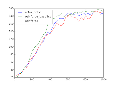
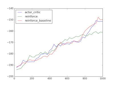
All 3 algorithms struggled with getting stuck in bad local optima on acrobot (around ~20% of the time). As a result, the averages are significantly lower than the best performing runs. This could be due to vanishing gradients or limitations of the efficacy of the policy gradient itself.

Extending the actor-critic policy gradient

Now that we’ve covered the basics of actor-critic methods, we can also motivate some of the more recent advances in deep reinforcement learning that built upon these ideas:

Deep Deterministic Policy Gradients which use DQN style updates to train an action-value function which acts as a critic. This greatly improves the sample efficiency of the stochastic policy gradient.
Trust Region Policy Optimization which restricts the policy gradient updates to a “trust region” determined by the KL divergence between the distributions predicted by the old and the new policy on a batch of data. TRPO has shown to perform extremely well on a wide variety of continuous control tasks with very little parameter tuning.
Asynchronous Actor-Critic (A3C) which parallelizes the sampling and policy gradient updates across multiple actor threads. This has a stabilizing effect on the gradient updates and leads to much faster training times.

Conclusion

In this post, we presented two types of actor-critic methods: REINFORCE with baseline and generalized advantage estimator actor-critic. We discussed why adding a baseline can stabilize the policy updates and reduce variance, at the cost of adding bias.

While our results for the GAE actor-critic did not yield significant gains over REINFORCE with baseline, it has been shown that the GAE actor-critic performs better than REINFORCE with baseline on harder continuous control problems. In future posts, we’ll discuss how policy gradient methods can be applied to continuous control environments using the reparameterization trick.